pacman::p_load(tidyverse, jsonlite,
               tidygraph, ggraph,
SmartEDA)MC3 Kickstarter
Overview
By the end of this hands-on exercise, you will be able to:
- import Mini Case 3 data file R object,
- split the knowledge graph into nodes and edges tibble data frames,
- tidy nodes and edges tibble data frames for conforming to the requirements of tidygraph,
- create a tidygrpah object by using the tidied nides and edges, and
- visualise the tidygraph
Getting Started
For the purpose of this exercise, five R packages will be used. They are tidyverse, jsonlite, tidygraph, ggraph and SmartEDA.
Note
You are required to install the R packages above, if necessary, before continue to the next step.
In the code chunk below, p_load() of pacman package is used to load the R packages into R environemnt.
Importing Knowledge Graph Data
For the purpose of this exercise, mc3.json file will be used. Before getting started, you should have the data set in the data sub-folder.
In the code chunk below, fromJSON() of jsonlite package is used to import mc3.json file into R and save the output object
MC3 <- fromJSON("data/MC3_graph.json")
MC3_schema <- fromJSON("data/MC3_schema.json")
Inspecting knowledge graph structure
Before preparing the data, it is always a good practice to examine the structure of mc3 knowledge graph.
In the code chunk below glimpse() is used to reveal the structure of mc3 knowledge graph.
glimpse(MC3)List of 5
$ directed : logi TRUE
$ multigraph: logi FALSE
$ graph :List of 4
..$ mode : chr "static"
..$ edge_default: Named list()
..$ node_default: Named list()
..$ name : chr "VAST_MC3_Knowledge_Graph"
$ nodes :'data.frame': 1159 obs. of 31 variables:
..$ type : chr [1:1159] "Entity" "Entity" "Entity" "Entity" ...
..$ label : chr [1:1159] "Sam" "Kelly" "Nadia Conti" "Elise" ...
..$ name : chr [1:1159] "Sam" "Kelly" "Nadia Conti" "Elise" ...
..$ sub_type : chr [1:1159] "Person" "Person" "Person" "Person" ...
..$ id : chr [1:1159] "Sam" "Kelly" "Nadia Conti" "Elise" ...
..$ timestamp : chr [1:1159] NA NA NA NA ...
..$ monitoring_type : chr [1:1159] NA NA NA NA ...
..$ findings : chr [1:1159] NA NA NA NA ...
..$ content : chr [1:1159] NA NA NA NA ...
..$ assessment_type : chr [1:1159] NA NA NA NA ...
..$ results : chr [1:1159] NA NA NA NA ...
..$ movement_type : chr [1:1159] NA NA NA NA ...
..$ destination : chr [1:1159] NA NA NA NA ...
..$ enforcement_type : chr [1:1159] NA NA NA NA ...
..$ outcome : chr [1:1159] NA NA NA NA ...
..$ activity_type : chr [1:1159] NA NA NA NA ...
..$ participants : int [1:1159] NA NA NA NA NA NA NA NA NA NA ...
..$ thing_collected :'data.frame': 1159 obs. of 2 variables:
.. ..$ type: chr [1:1159] NA NA NA NA ...
.. ..$ name: chr [1:1159] NA NA NA NA ...
..$ reference : chr [1:1159] NA NA NA NA ...
..$ date : chr [1:1159] NA NA NA NA ...
..$ time : chr [1:1159] NA NA NA NA ...
..$ friendship_type : chr [1:1159] NA NA NA NA ...
..$ permission_type : chr [1:1159] NA NA NA NA ...
..$ start_date : chr [1:1159] NA NA NA NA ...
..$ end_date : chr [1:1159] NA NA NA NA ...
..$ report_type : chr [1:1159] NA NA NA NA ...
..$ submission_date : chr [1:1159] NA NA NA NA ...
..$ jurisdiction_type: chr [1:1159] NA NA NA NA ...
..$ authority_level : chr [1:1159] NA NA NA NA ...
..$ coordination_type: chr [1:1159] NA NA NA NA ...
..$ operational_role : chr [1:1159] NA NA NA NA ...
$ edges :'data.frame': 3226 obs. of 5 variables:
..$ id : chr [1:3226] "2" "3" "5" "3013" ...
..$ is_inferred: logi [1:3226] TRUE FALSE TRUE TRUE TRUE TRUE ...
..$ source : chr [1:3226] "Sam" "Sam" "Sam" "Sam" ...
..$ target : chr [1:3226] "Relationship_Suspicious_217" "Event_Communication_370" "Event_Assessment_600" "Relationship_Colleagues_430" ...
..$ type : chr [1:3226] NA "sent" NA NA ...
Warning
Notice that Industry field is in list data type. In general, this data type is not acceptable by tbl_graph() of tidygraph. In order to avoid error arise when building tidygraph object, it is wiser to exclude this field from the edges data table. However, it might be still useful in subsequent analysis.
Extracting the edges and nodes tables
Next, as_tibble() of tibble package package is used to extract the nodes and links tibble data frames from mc3 tibble dataframe into two separate tibble dataframes called mc3_nodes and mc3_edges respectively.
mc3_nodes <- as_tibble(MC3$nodes)
mc3_edges <- as_tibble(MC3$edges)
Initial EDA
It is time for us to apply appropriate EDA methods to examine the data.
In the code chunk below, ExpCatViz() of SmartEDA package is used to reveal the frequency distribution of all categorical fields in mc3_nodes tibble dataframe.
ExpCatViz(data=mc3_nodes,
          col="lightblue")
[[1]]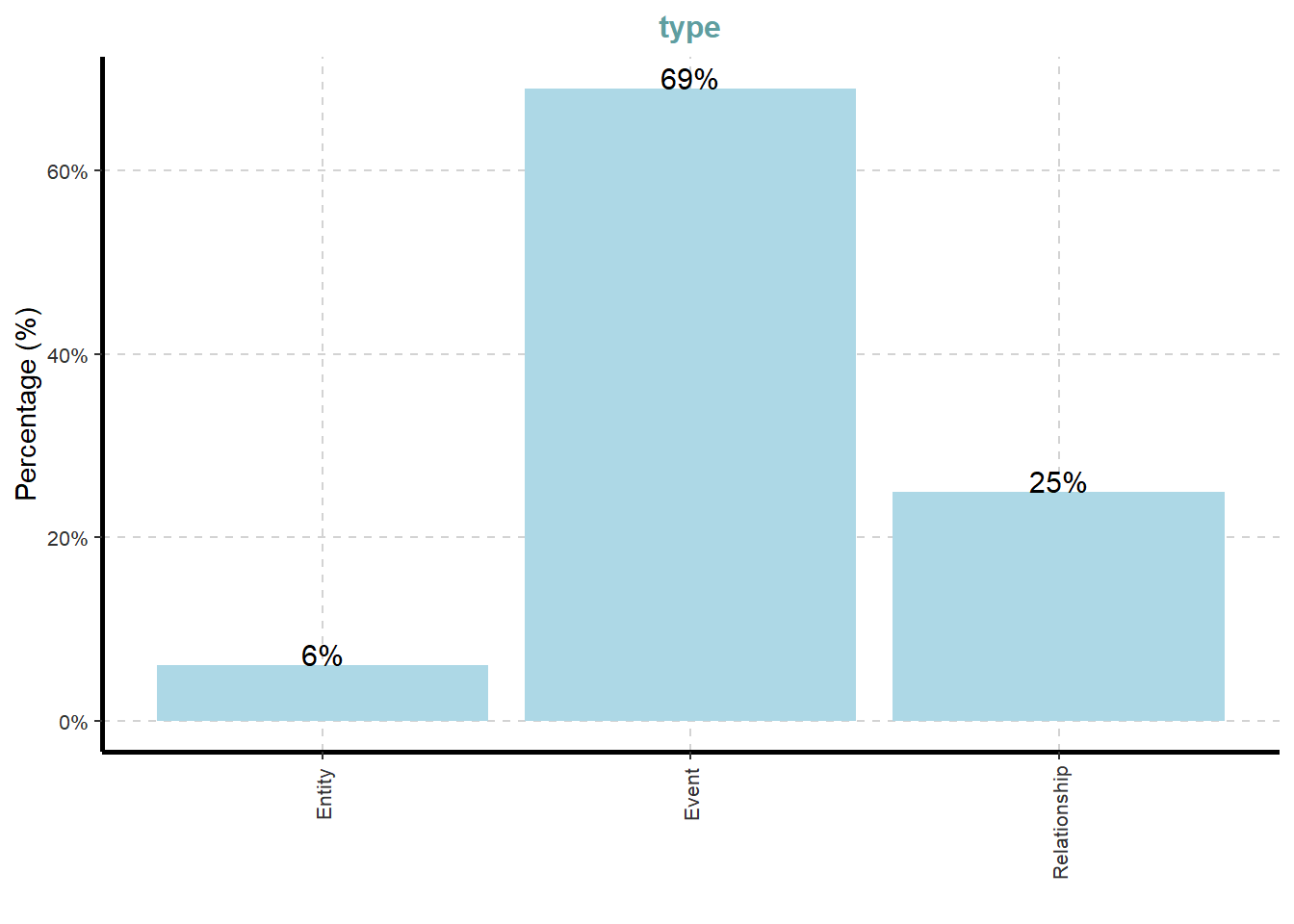
[[2]]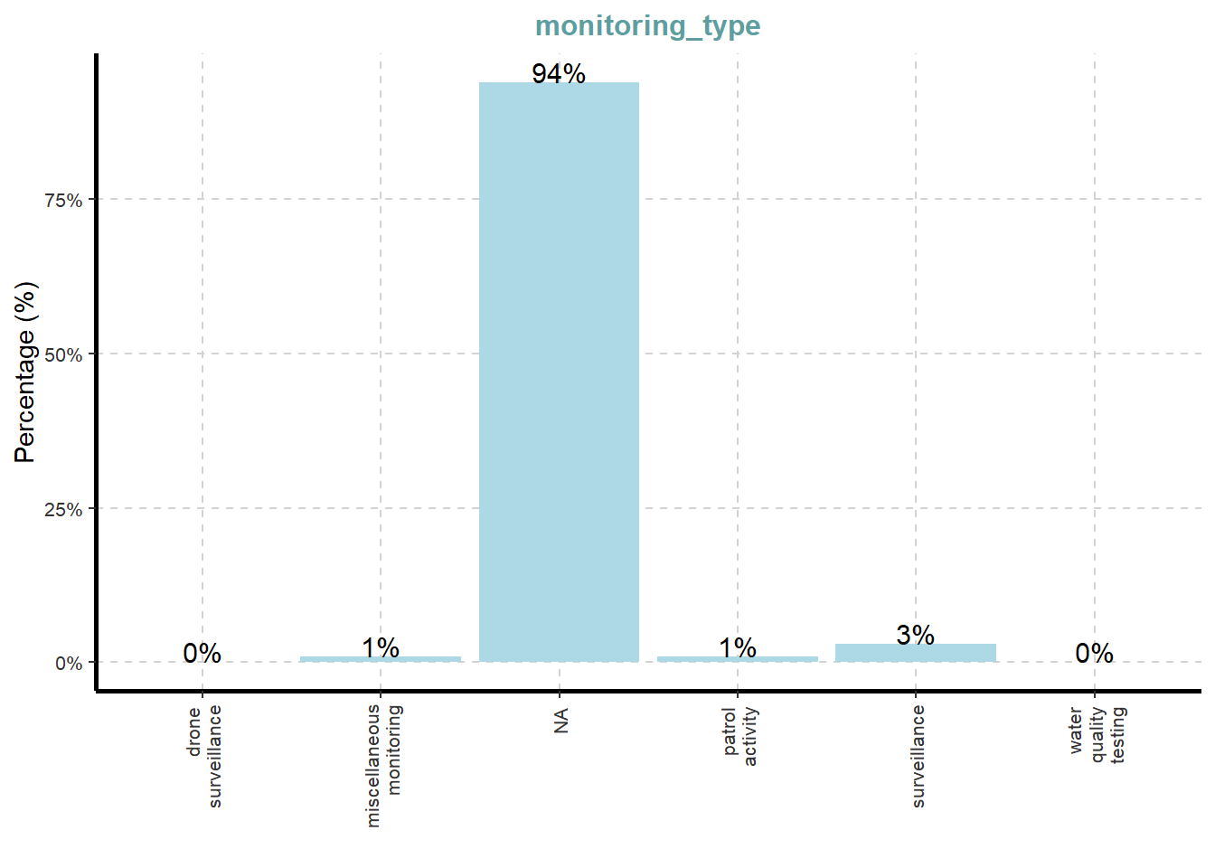
[[3]]
[[4]]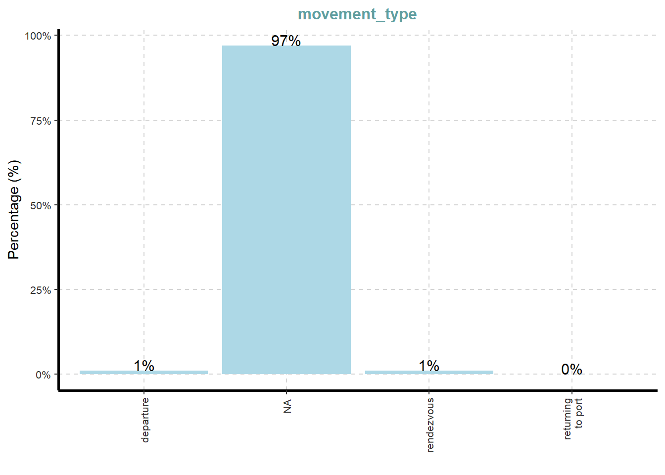
[[5]]
[[6]]
[[7]]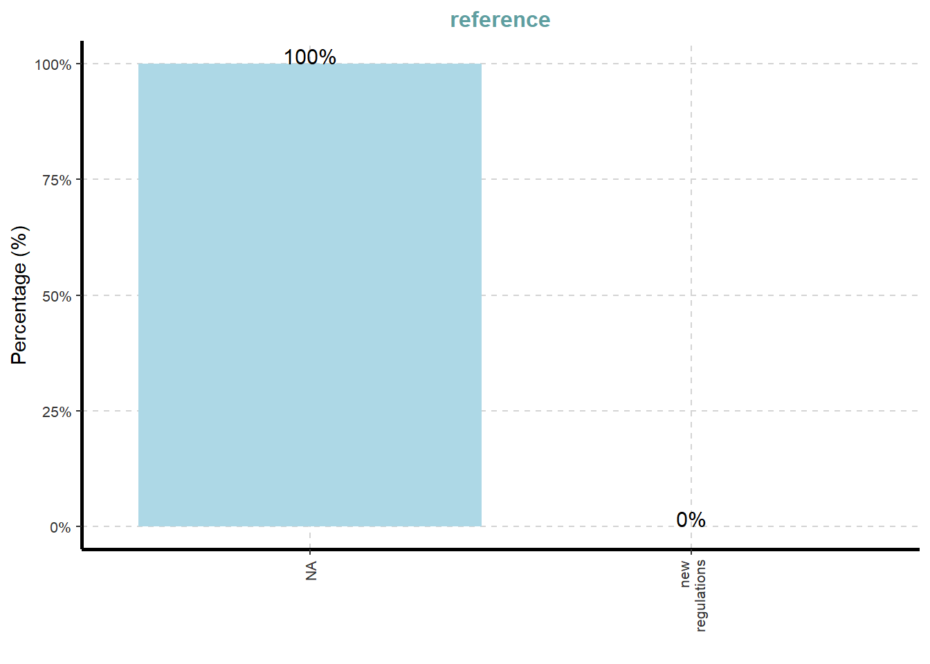
[[8]]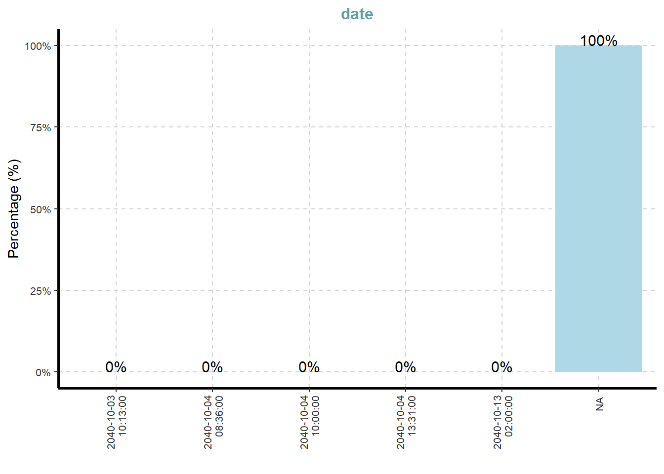
[[9]]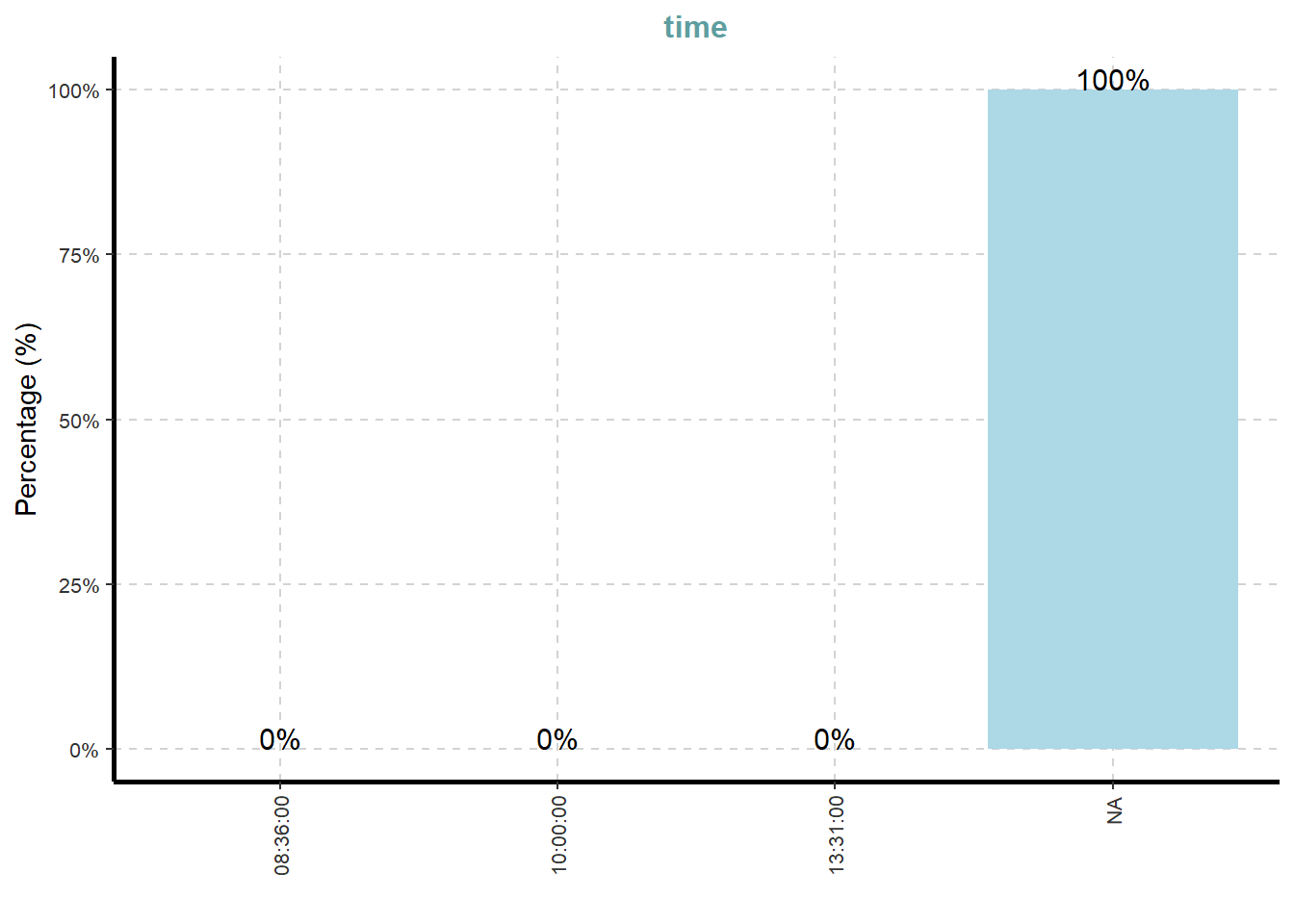
[[10]]
[[11]]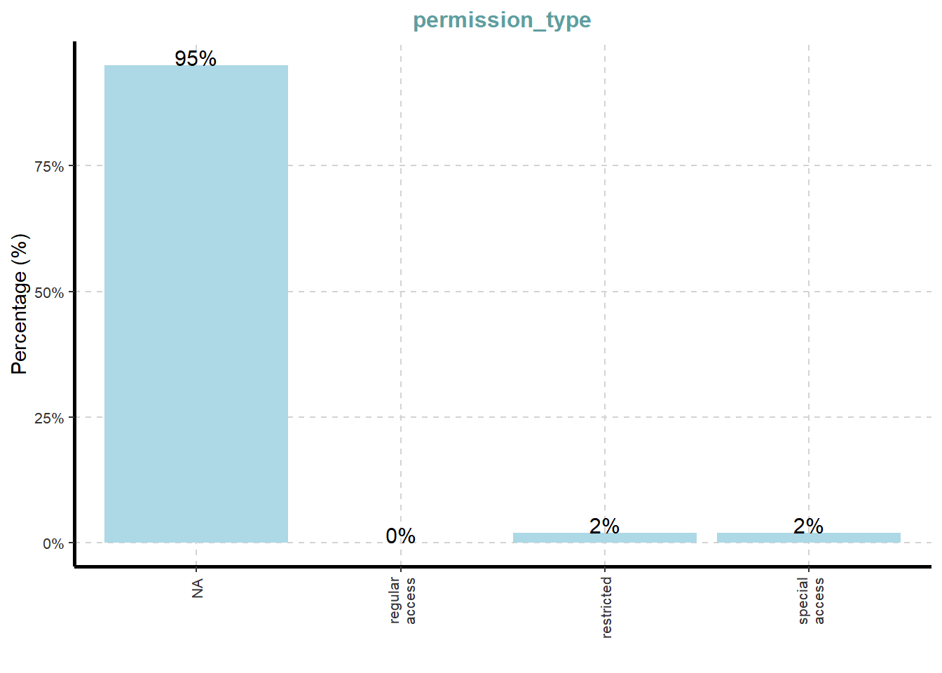
[[12]]
[[13]]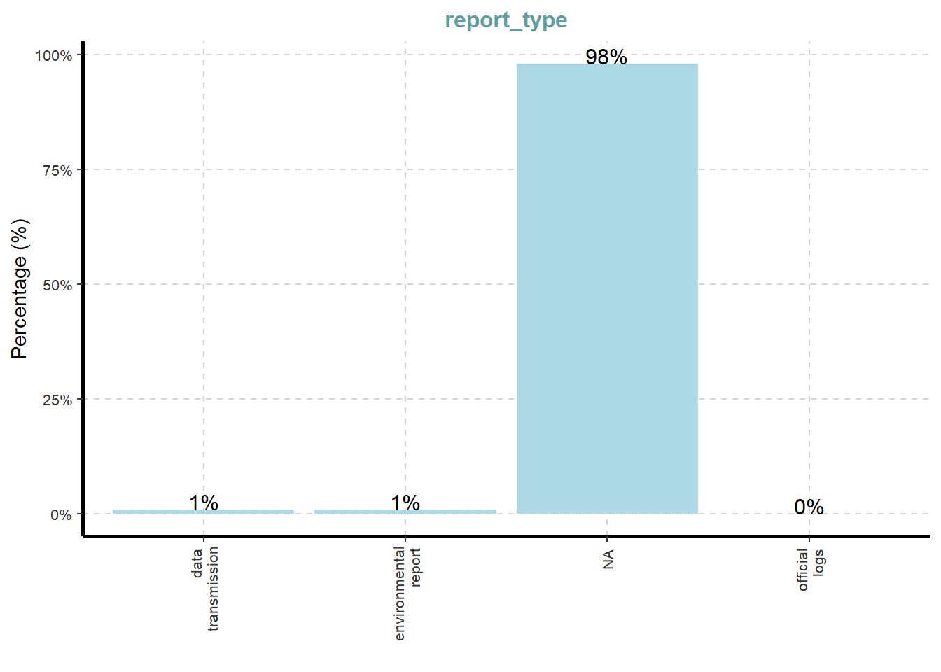
[[14]]
Note
What useful discovery can you obtained from the visualisation above?
On the other hands, code chunk below uses ExpCATViz() of SmartEDA package to reveal the frequency distribution of all categorical fields in mc3_edges tibble dataframe.
ExpCatViz(data=mc3_edges,
          col="lightblue")
[[1]]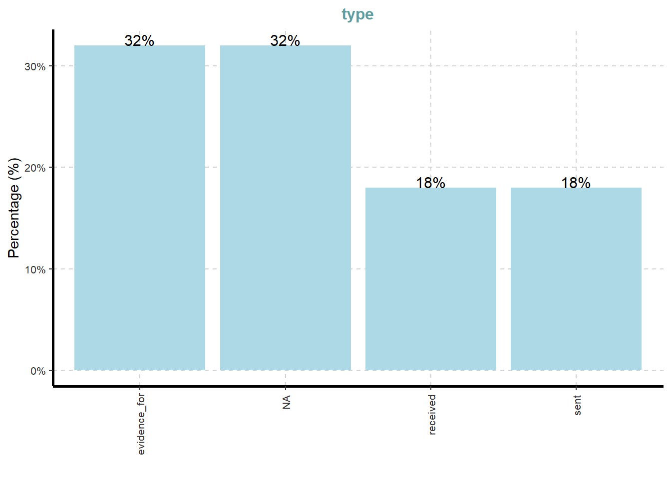
Note
What useful discovery can you obtained from the visualisation above?
Data Cleaning and Wrangling
Cleaning and wrangling nodes
Code chunk below performs the following data cleaning tasks:
- convert values in id field into character data type,
- exclude records with
idvalue are na, - exclude records with similar id values,
- exclude
thing_collectedfield, and - save the cleaned tibble dataframe into a new tibble datatable called
mc3_nodes_cleaned.
mc3_nodes_cleaned <- mc3_nodes %>%
  mutate(id = as.character(id)) %>%
  filter(!is.na(id)) %>%
  distinct(id, .keep_all = TRUE) %>%
  select(-thing_collected)
Cleaning and wrangling edges
Next, the code chunk below will be used to:
- rename source and target fields to from_id and to_id respectively,
- convert values in from_id and to_id fields to character data type,
- exclude values in from_id and to_id which not found in the id field of mc3_nodes_cleaned,
- exclude records whereby from_id and/or to_id values are missing, and
- save the cleaned tibble dataframe and called it mc3_edges_cleaned.
mc3_edges_cleaned <- mc3_edges %>%
  rename(from_id = source,
         to_id = target) %>%
  mutate(across(c(from_id, to_id),
                as.character)) %>%
  filter(from_id %in% mc3_nodes_cleaned$id,
         to_id %in% mc3_nodes_cleaned$id) %>%
  filter(!is.na(from_id), !is.na(to_id))
Next, code chunk below will be used to create mapping of character id in mc3_nodes_cleaned to row index
node_index_lookup <- mc3_nodes_cleaned %>%
  mutate(.row_id = row_number()) %>%
  select(id, .row_id)
Next, the code chunk below will be used to join and convert from_id and to_id to integer indices. At the same time we also drop rows with unmatched nodes.
mc3_edges_indexed <- mc3_edges_cleaned %>%
  left_join(node_index_lookup,
            by = c("from_id" = "id")) %>%
  rename(from = .row_id) %>%
  left_join(node_index_lookup,
            by = c("to_id" = "id")) %>%
  rename(to = .row_id) %>%
  select(from, to, is_inferred, type) %>%
  filter(!is.na(from) & !is.na(to))
Next the code chunk below is used to subset nodes to only those referenced by edges.
used_node_indices <- sort(
  unique(c(mc3_edges_indexed$from,
           mc3_edges_indexed$to)))

mc3_nodes_final <- mc3_nodes_cleaned %>%
  slice(used_node_indices) %>%
  mutate(new_index = row_number())
We will then use the code chunk below to rebuild lookup from old index to new index.
old_to_new_index <- tibble(
  old_index = used_node_indices,
  new_index = seq_along(
    used_node_indices))
Lastly, the code chunk below will be used to update edge indices to match new node table.
mc3_edges_final <- mc3_edges_indexed %>%
  left_join(old_to_new_index,
            by = c("from" = "old_index")) %>%
  rename(from_new = new_index) %>%
  left_join(old_to_new_index,
            by = c("to" = "old_index")) %>%
  rename(to_new = new_index) %>%
  select(from = from_new, to = to_new,
         is_inferred, type)
Building the tidygraph object
Now we are ready to build the tidygraph object by using the code chunk below.
mc3_graph <- tbl_graph(
  nodes = mc3_nodes_final,
  edges = mc3_edges_final,
  directed = TRUE
)
After the tidygraph object is created, it is always a good practice to examine the object by using str().
str(mc3_graph)Classes 'tbl_graph', 'igraph' hidden list of 10
$ : num 1159
$ : logi TRUE
$ : num [1:3226] 0 0 0 0 0 0 0 1 1 1 ...
$ : num [1:3226] 1137 356 746 894 875 ...
$ : NULL
$ : NULL
$ : NULL
$ : NULL
$ :List of 4
..$ : num [1:3] 1 0 1
..$ : Named list()
..$ :List of 31
.. ..$ type : chr [1:1159] "Entity" "Entity" "Entity" "Entity" ...
.. ..$ label : chr [1:1159] "Sam" "Kelly" "Nadia Conti" "Elise" ...
.. ..$ name : chr [1:1159] "Sam" "Kelly" "Nadia Conti" "Elise" ...
.. ..$ sub_type : chr [1:1159] "Person" "Person" "Person" "Person" ...
.. ..$ id : chr [1:1159] "Sam" "Kelly" "Nadia Conti" "Elise" ...
.. ..$ timestamp : chr [1:1159] NA NA NA NA ...
.. ..$ monitoring_type : chr [1:1159] NA NA NA NA ...
.. ..$ findings : chr [1:1159] NA NA NA NA ...
.. ..$ content : chr [1:1159] NA NA NA NA ...
.. ..$ assessment_type : chr [1:1159] NA NA NA NA ...
.. ..$ results : chr [1:1159] NA NA NA NA ...
.. ..$ movement_type : chr [1:1159] NA NA NA NA ...
.. ..$ destination : chr [1:1159] NA NA NA NA ...
.. ..$ enforcement_type : chr [1:1159] NA NA NA NA ...
.. ..$ outcome : chr [1:1159] NA NA NA NA ...
.. ..$ activity_type : chr [1:1159] NA NA NA NA ...
.. ..$ participants : int [1:1159] NA NA NA NA NA NA NA NA NA NA ...
.. ..$ reference : chr [1:1159] NA NA NA NA ...
.. ..$ date : chr [1:1159] NA NA NA NA ...
.. ..$ time : chr [1:1159] NA NA NA NA ...
.. ..$ friendship_type : chr [1:1159] NA NA NA NA ...
.. ..$ permission_type : chr [1:1159] NA NA NA NA ...
.. ..$ start_date : chr [1:1159] NA NA NA NA ...
.. ..$ end_date : chr [1:1159] NA NA NA NA ...
.. ..$ report_type : chr [1:1159] NA NA NA NA ...
.. ..$ submission_date : chr [1:1159] NA NA NA NA ...
.. ..$ jurisdiction_type: chr [1:1159] NA NA NA NA ...
.. ..$ authority_level : chr [1:1159] NA NA NA NA ...
.. ..$ coordination_type: chr [1:1159] NA NA NA NA ...
.. ..$ operational_role : chr [1:1159] NA NA NA NA ...
.. ..$ new_index : int [1:1159] 1 2 3 4 5 6 7 8 9 10 ...
..$ :List of 2
.. ..$ is_inferred: logi [1:3226] TRUE FALSE TRUE TRUE TRUE TRUE ...
.. ..$ type : chr [1:3226] NA "sent" NA NA ...
$ :<environment: 0x000002835e7a4a20>
- attr(*, "active")= chr "nodes"Visualising the knowledge graph
Several of the ggraph layouts involve randomisation. In order to ensure reproducibility, it is necessary to set the seed value before plotting by using the code chunk below.
set.seed(1234)In the code chunk below, ggraph functions are used to create the whole graph.
ggraph(mc3_graph,
       layout = "fr") +
  geom_edge_link(alpha = 0.3,
                 colour = "gray") +
  geom_node_point(aes(color = `type`),
                  size = 4) +
  geom_node_text(aes(label = type),
                 repel = TRUE,
                 size = 2.5) +
  theme_void()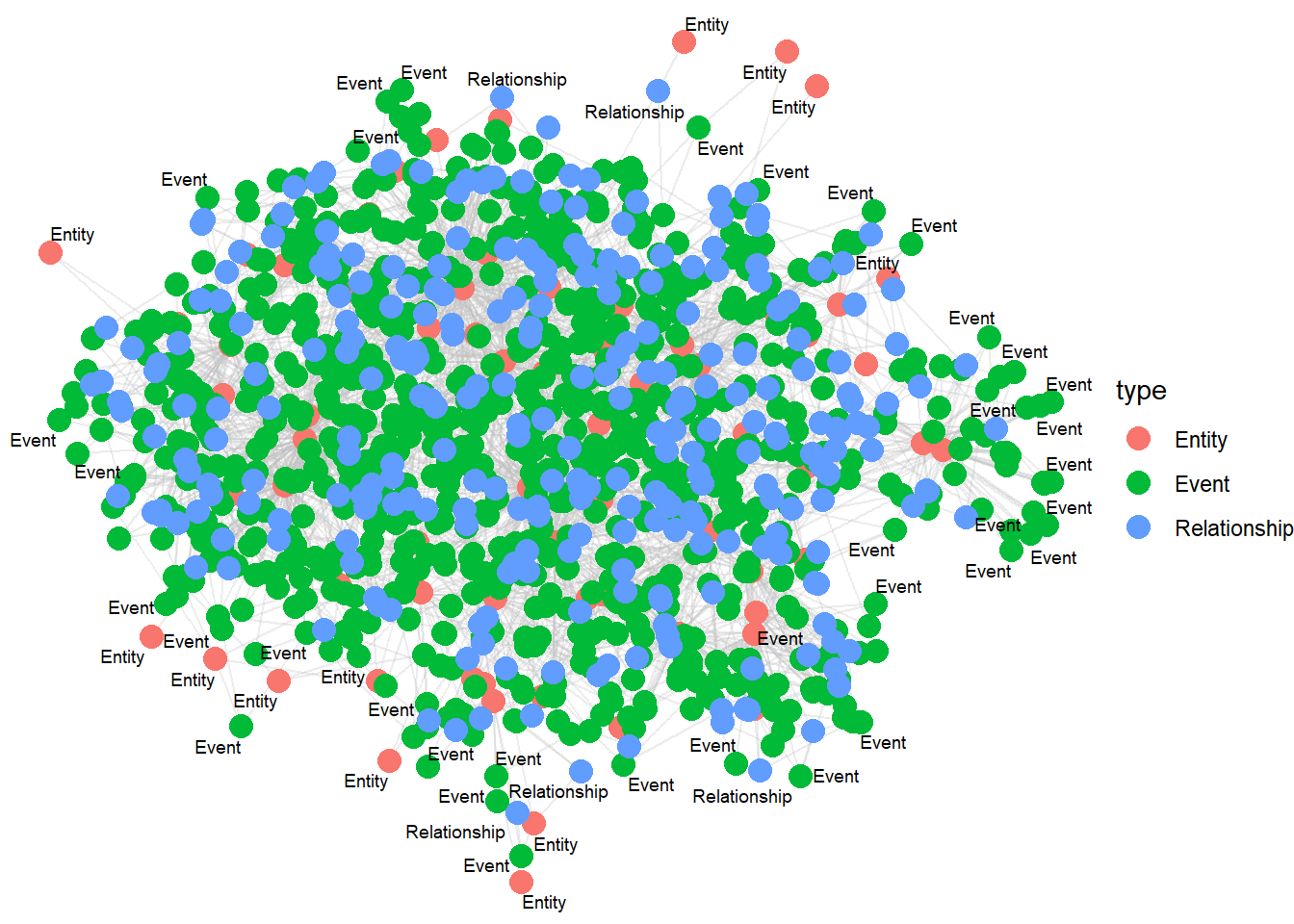
Warning
The example below is not model answers, It is used to show you how to use the mantra of Overview first, details on demand of visual investigation.