MC2 Kickstarter

Published

May 12, 2025

Modified

May 20, 2025

Overview

By the end of this hands-on exercise, you will be able to:

import Mini Case 2 data file R object,
split the knowledge graph into nodes and edges tibble data frames,
tidy nodes and edges tibble data frames for conforming to the requirements of tidygraph,
create a tidygrpah object by using the tidied nides and edges, and
visualise the tidygraph

Getting Started

For the purpose of this exercise, five R packages will be used. They are tidyverse, jsonlite, tidygraph, ggraph and SmartEDA.

Note

You are required to install the R packages above, if necessary, before continue to the next step.

In the code chunk below, p_load() of pacman package is used to load the R packages into R environemnt.

pacman::p_load(tidyverse, jsonlite,
               tidygraph, ggraph,
               SmartEDA)

Importing Knowledge Graph Data

For the purpose of this exercise, FILAH.json file will be used. Before getting started, you should have the data set in the data sub-folder.

In the code chunk below, fromJSON() of jsonlite package is used to import FILAH.json file into R and save the output object

filah <- fromJSON("data/FILAH.json")

Inspecting knowledge graph structure

Before preparing the data, it is always a good practice to examine the structure of filah knowledge graph.

In the code chunk below glimpse() is used to reveal the structure of filah knowledge graph.

glimpse(filah)

List of 5
 $ directed  : logi TRUE
 $ multigraph: logi TRUE
 $ graph     : Named list()
 $ nodes     :'data.frame': 396 obs. of  17 variables:
  ..$ type       : chr [1:396] "meeting" "meeting" "meeting" "meeting" ...
  ..$ date       : chr [1:396] "Meeting 1" "Meeting 2" "Meeting 3" "Meeting 4" ...
  ..$ label      : chr [1:396] "Meeting 1" "Meeting 2" "Meeting 3" "Meeting 4" ...
  ..$ id         : chr [1:396] "Meeting_1" "Meeting_2" "Meeting_3" "Meeting_4" ...
  ..$ name       : chr [1:396] NA NA NA NA ...
  ..$ role       : chr [1:396] NA NA NA NA ...
  ..$ short_topic: chr [1:396] NA NA NA NA ...
  ..$ long_topic : chr [1:396] NA NA NA NA ...
  ..$ short_title: chr [1:396] NA NA NA NA ...
  ..$ long_title : chr [1:396] NA NA NA NA ...
  ..$ plan_type  : chr [1:396] NA NA NA NA ...
  ..$ lat        : num [1:396] NA NA NA NA NA NA NA NA NA NA ...
  ..$ lon        : num [1:396] NA NA NA NA NA NA NA NA NA NA ...
  ..$ zone       : chr [1:396] NA NA NA NA ...
  ..$ zone_detail: chr [1:396] NA NA NA NA ...
  ..$ start      : chr [1:396] NA NA NA NA ...
  ..$ end        : chr [1:396] NA NA NA NA ...
 $ links     :'data.frame': 765 obs. of  9 variables:
  ..$ role     : chr [1:765] "part_of" "part_of" "part_of" "part_of" ...
  ..$ source   : chr [1:765] "Meeting_1" "Meeting_1" "Meeting_1" "Meeting_1" ...
  ..$ target   : chr [1:765] "fish_vacuum_Meeting_1_Introduction_Discussion" "fish_vacuum_Meeting_1_Introduction" "seafood_festival_Meeting_1_Discussion" "seafood_festival_Meeting_1_Feasibility" ...
  ..$ key      : int [1:765] 0 0 0 0 0 0 0 0 0 0 ...
  ..$ sentiment: num [1:765] NA NA NA NA NA NA NA NA NA NA ...
  ..$ reason   : chr [1:765] NA NA NA NA ...
  ..$ industry :List of 765
  .. ..$ : NULL
  .. ..$ : NULL
  .. ..$ : NULL
  .. ..$ : NULL
  .. ..$ : NULL
  .. ..$ : NULL
  .. ..$ : NULL
  .. ..$ : NULL
  .. ..$ : NULL
  .. ..$ : NULL
  .. ..$ : NULL
  .. ..$ : NULL
  .. ..$ : NULL
  .. ..$ : NULL
  .. ..$ : NULL
  .. ..$ : NULL
  .. ..$ : NULL
  .. ..$ : NULL
  .. ..$ : NULL
  .. ..$ : NULL
  .. ..$ : NULL
  .. ..$ : NULL
  .. ..$ : NULL
  .. ..$ : NULL
  .. ..$ : NULL
  .. ..$ : NULL
  .. ..$ : NULL
  .. ..$ : NULL
  .. ..$ : NULL
  .. ..$ : NULL
  .. ..$ : NULL
  .. ..$ : NULL
  .. ..$ : NULL
  .. ..$ : NULL
  .. ..$ : NULL
  .. ..$ : NULL
  .. ..$ : NULL
  .. ..$ : NULL
  .. ..$ : NULL
  .. ..$ : NULL
  .. ..$ : NULL
  .. ..$ : NULL
  .. ..$ : NULL
  .. ..$ : NULL
  .. ..$ : NULL
  .. ..$ : NULL
  .. ..$ : NULL
  .. ..$ : NULL
  .. ..$ : NULL
  .. ..$ : NULL
  .. ..$ : NULL
  .. ..$ : NULL
  .. ..$ : NULL
  .. ..$ : NULL
  .. ..$ : NULL
  .. ..$ : NULL
  .. ..$ : NULL
  .. ..$ : NULL
  .. ..$ : NULL
  .. ..$ : NULL
  .. ..$ : NULL
  .. ..$ : NULL
  .. ..$ : NULL
  .. ..$ : NULL
  .. ..$ : NULL
  .. ..$ : NULL
  .. ..$ : NULL
  .. ..$ : NULL
  .. ..$ : NULL
  .. ..$ : NULL
  .. ..$ : NULL
  .. ..$ : NULL
  .. ..$ : NULL
  .. ..$ : NULL
  .. ..$ : NULL
  .. ..$ : NULL
  .. ..$ : NULL
  .. ..$ : NULL
  .. ..$ : NULL
  .. ..$ : NULL
  .. ..$ : NULL
  .. ..$ : NULL
  .. ..$ : NULL
  .. ..$ : NULL
  .. ..$ : NULL
  .. ..$ : NULL
  .. ..$ : NULL
  .. ..$ : NULL
  .. ..$ : NULL
  .. ..$ : NULL
  .. ..$ : NULL
  .. ..$ : NULL
  .. ..$ : NULL
  .. ..$ : NULL
  .. ..$ : NULL
  .. ..$ : NULL
  .. ..$ : NULL
  .. ..$ : NULL
  .. ..$ : NULL
  .. .. [list output truncated]
  ..$ status   : chr [1:765] NA NA NA NA ...
  ..$ time     : chr [1:765] NA NA NA NA ...

Warning

Notice that Industry field is in list data type. In general, this data type is not acceptable by tbl_graph() of tidygraph. In order to avoid error arise when building tidygraph object, it is wiser to exclude this field from the edges data table. However, it might be still useful in subsequent analysis.

Extracting the edges and nodes tables

Next, as_tibble() of tibble package package is used to extract the nodes and links tibble data frames from filah tibble dataframe into two separate tibble dataframes called filah_nodes and filah_edges respectively.

filah_nodes <- as_tibble(filah$nodes)
filah_edges <- as_tibble(filah$links)

Initial EDA

It is time for us to apply appropriate EDA methods to examine the data.

In the code chunk below, ExpCatViz() of SmartEDA package is used to reveal the frequency distribution of all categorical fields in filah_nodes tibble dataframe.

ExpCatViz(data=filah_nodes,
          col="lightblue")

[[1]]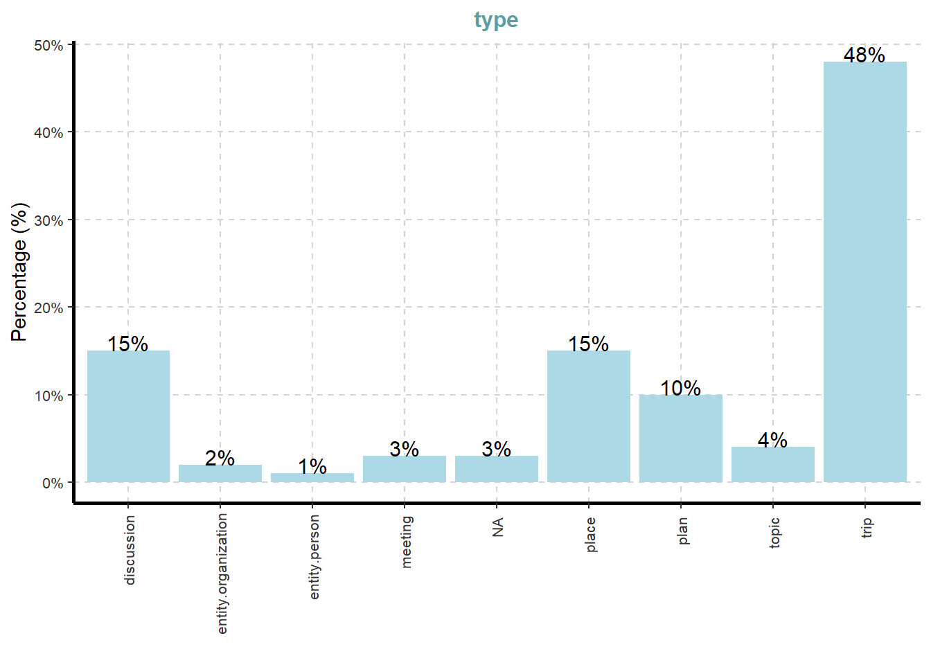


[[2]]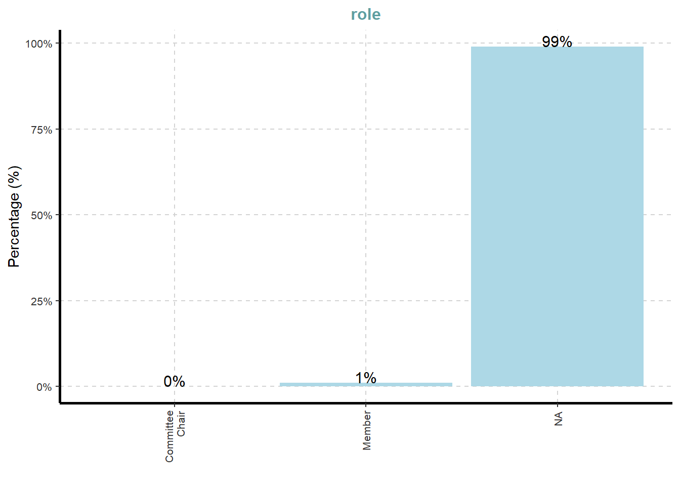


[[3]]


[[4]]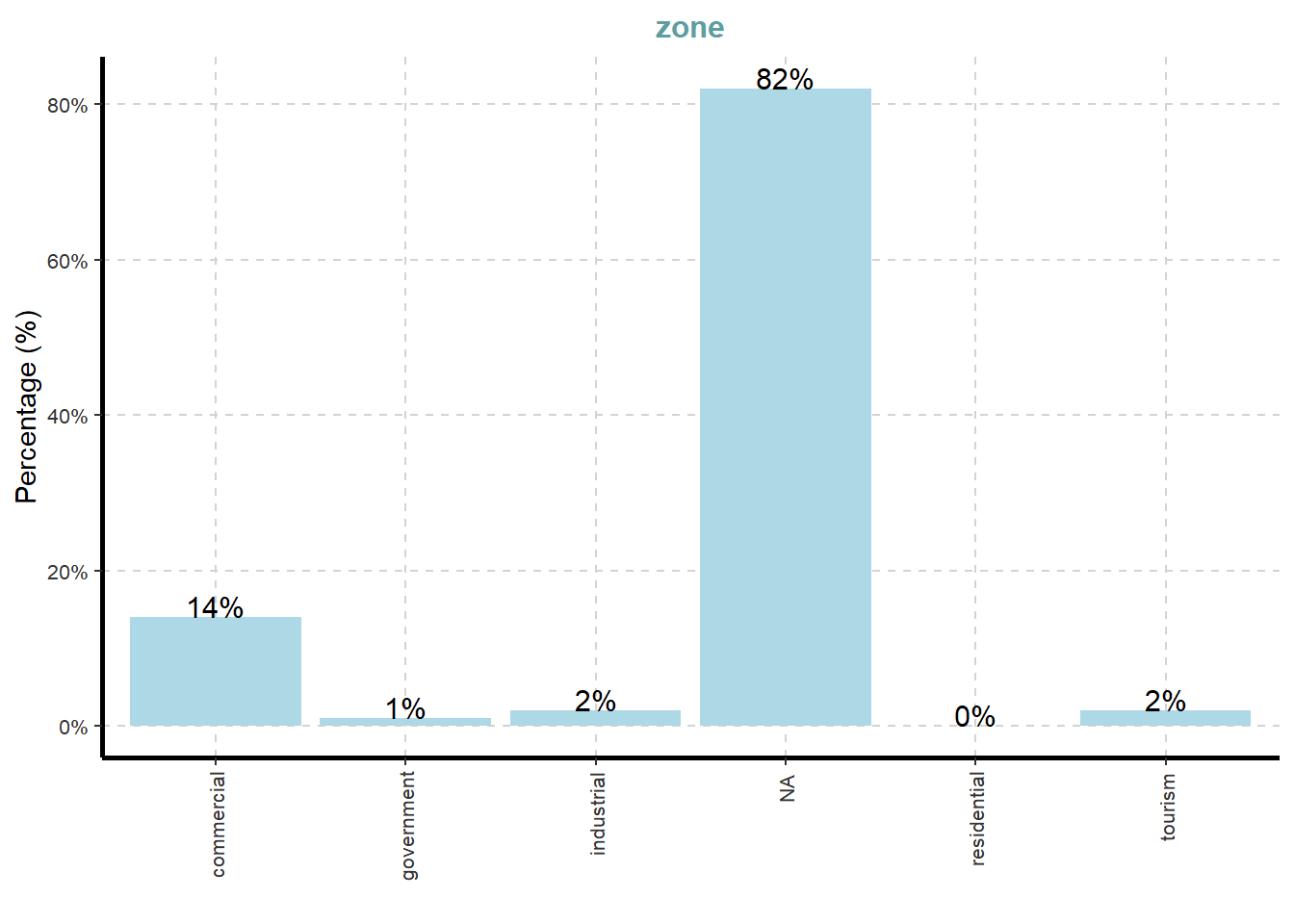


[[5]]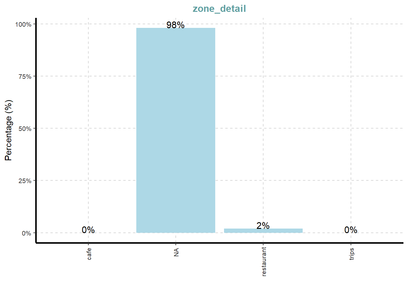

Note

What useful discovery can you obtained from the visualisation above?

On the other hands, code chunk below uses ExpCATViz() of SmartEDA package to reveal the frequency distribution of all categorical fields in filah_edges tibble dataframe.

ExpCatViz(data=filah_edges,
          col="lightblue")

[[1]]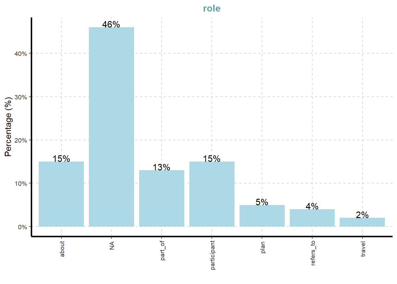


[[2]]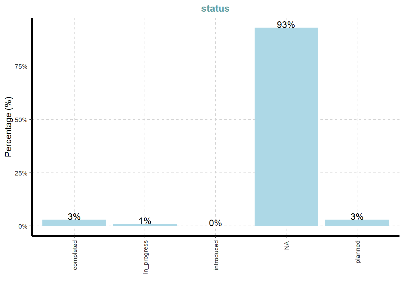


[[3]]

Note

What useful discovery can you obtained from the visualisation above?

ExpNumViz(filah_nodes)

[[1]]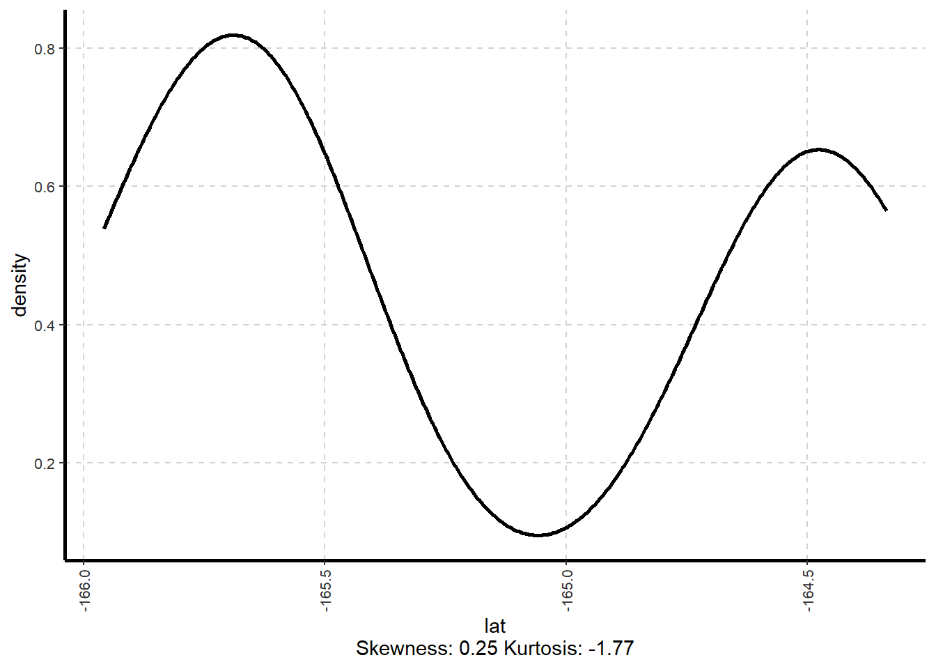


[[2]]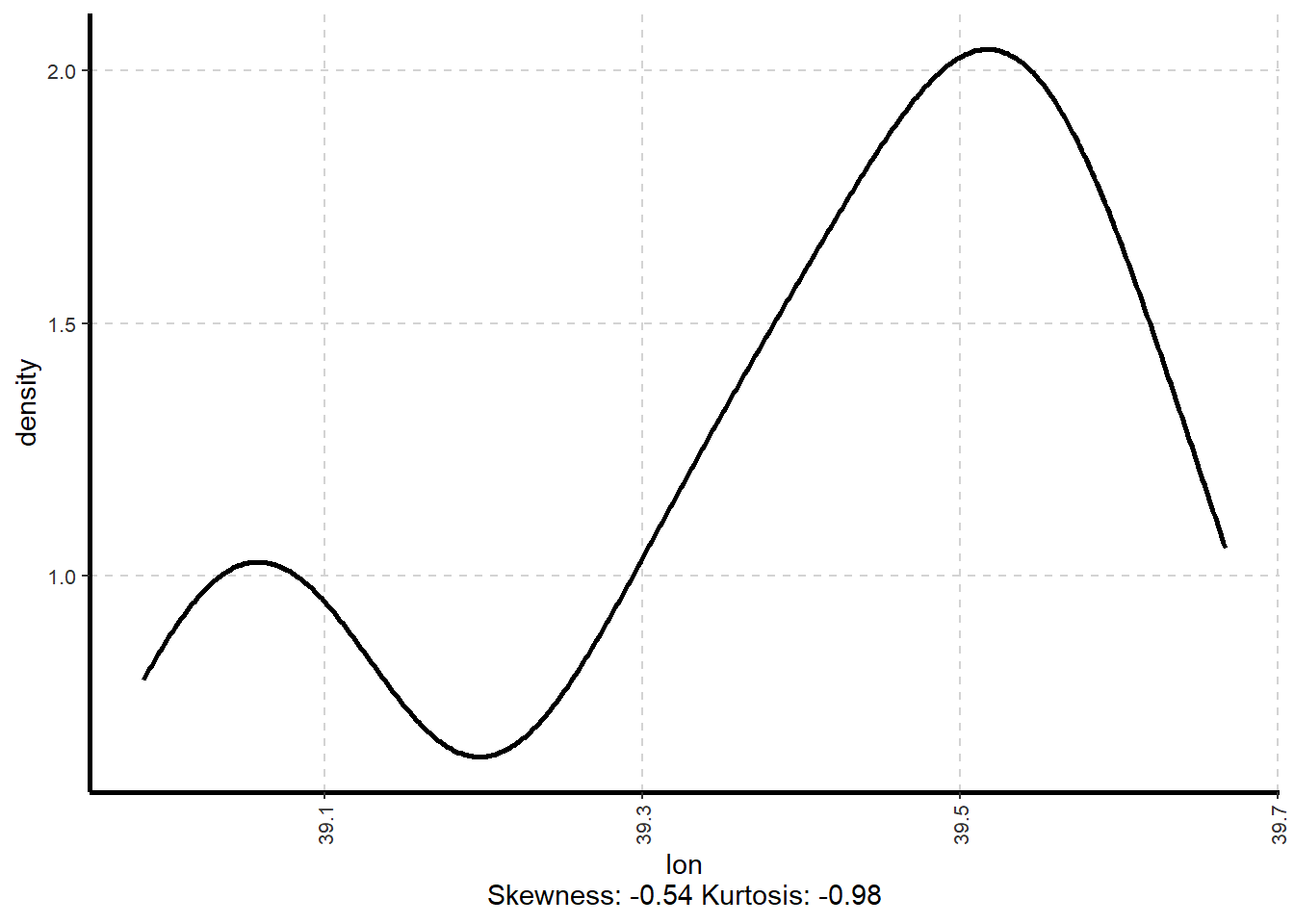

Note

What useful discovery can you obtained from the visualisation above?

ExpNumViz(filah_edges)

[[1]]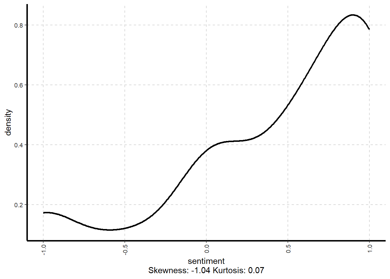

Note

What useful discovery can you obtained from the visualisation above?

Data Cleaning and Wrangling

Cleaning and wrangling nodes

filah_nodes_cleaned <- filah_nodes %>%
  mutate(id = as.character(id)) %>%
  filter(!is.na(id)) %>%
  distinct(id, .keep_all = TRUE) %>%
  select(id, type, label)

Cleaning and wrangling edges

filah_edges_cleaned <- filah_edges %>%
  rename(from = source, to = target) %>%
  mutate(across(c(from, to), as.character)) %>%
  filter(from %in% filah_nodes_cleaned$id, to %in% filah_nodes_cleaned$id)

# Remove problematic columns from edge table for graph building
filah_edges_min <- filah_edges_cleaned %>%
  select(from, to, role)  # Only basic fields needed for graph structure

Building the tidygraph object

filah_graph <- tbl_graph(
  nodes = filah_nodes_cleaned, 
  edges = filah_edges_min, 
  directed = TRUE)

Note

Since the similar steps will be used to clean and wrangle TROUT.json and journalist.json, you might want to consider converting the above code chunks into R function(s).

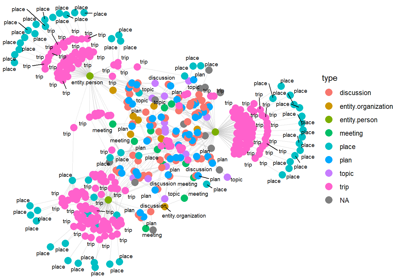
Visualising the knowledge graph

In this section, we will use ggraph’s functions to visualise and analyse the graph object.

Warning

The example below is not model answers, It is used to show you how to use the mantra of Overview first, details on demand of visual investigation.

Visualising the whole graph

Several of the ggraph layouts involve randomisation. In order to ensure reproducibility, it is necessary to set the seed value before plotting by using the code chunk below.

set.seed(1234)

In the code chunk below, ggraph functions are used to create the whole graph.

ggraph(filah_graph, 
       layout = "fr") +
  geom_edge_link(alpha = 0.3, 
                 colour = "gray") +
  geom_node_point(aes(color = `type`), 
                  size = 4) +
  geom_node_text(aes(label = type), 
                 repel = TRUE, 
                 size = 2.5) +
  theme_void()